Deep Dive: YOLO In-and-Out Part 1 - from V1 to V4!
Advanced Machine Learning
Today we deep dive into YOLO (You Only Look Once) the state-of-the-art model for real-time object detection. Since the first version in 2015, a lot of improvements have been made and it quickly became the default approach for real-time object detection. Today we only cover half of the work as too much has been done to go over everything at once. We cover:
What is YOLO?
YOLO V1
YOLO V2
YOLO V3
YOLO V4
What is YOLO?
YOLO stands for "You Only Look Once"! It was first published in 2015 and quickly became the State of the art of real-time object detection. Unlike previous methods that involved running a classifier on many different patches of an image, YOLO applies the detection to the whole image at once.
YOLO has multiple versions, from YOLOv1 to YOLOv8. Each version introduces improvements over the previous ones in terms of detection accuracy, speed, or both. One key advantage of YOLO over other object detection methods is its speed, making it suitable for real-time object detection tasks. However, it tends to be less accurate with small objects and objects that are close together due to the grid system it uses.
The first version of YOLO was published in 2015 by Joseph Redmon and a few other people. It introduced for the first time the possibility of detecting objects in real time. Redmon and Ali Farhadi developed further YOLO V2 in 2016 and YOLO V3 in 2018. Among other things, YOLO V2 introduced anchor boxes, the Darknet-19 architecture, and fully convolutional predictions. V3 used the Darknet-53 architecture and multi-scale predictions.
In 2020 Redmon announced that he stopped doing CV research due to the military applications and that was when other teams started to take over his legacy! In 2020, Alexey Bochkovskiy et al. published the V4 paper with more emphasis on optimizing the network hyperparameters and an IOU-based loss function.
YOLO V1
Labeling the data
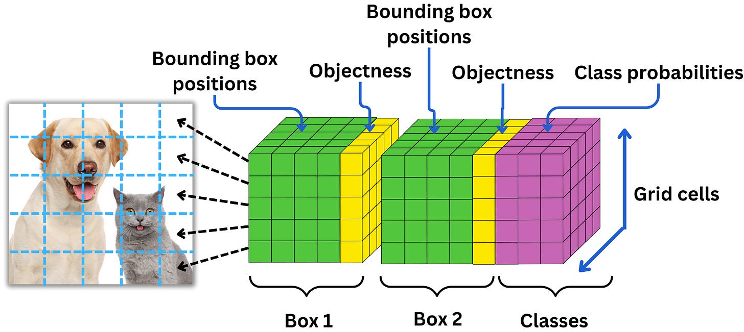
The idea is to segment the image into a grid and predict the existence of bounding boxes for the classes we are considering. In YOLO v1 the grid size is 7 x 7. When it comes to labeling the data, a grid cell is labeled to contain an object only if the center of the bounding box is in it. If the grid cell contains a center, the "objectness" is labeled 1 and 0 otherwise. The model will try to predict the probability that a grid cell contains a center. If it contains a center, each class related to those centers will be labeled with 1s.
If we have 2 classes (e.g. cat and dog), the label vector will be [1, 1, 0] if the grid cell contains a cat. In the case the grid cell contains a cat and a dog, we need to choose one of the classes as the label for the training data. Added to that, the label vector holds as well the (x, y) coordinates of the bounding box centers from the top left corner of the grid cell and their sizes (w, h) relative to the full image : [x, y, w, h, 1, 1, 0].
The prediction tensor
For each grid cell, the model will predict parameters for B boxes (for V1, we have B = 2). For each box, the model predicts x, y, w, and h along with the probability p that there is an object in that box. Along with the box’s predictions, the model predicts a probability for each of the classes. For each box, we predict 5 parameters and for each class, we predict 1 parameter, so for each grid cell we predict B x 5 + C where C is the number of classes. The overall number of parameters is
where S x S is the grid size.
If we call P(object) the probability there is an object in a box b and P(c|object) the probability that the object is of class c, then the score for the class c in the box b in simply
The Architecture
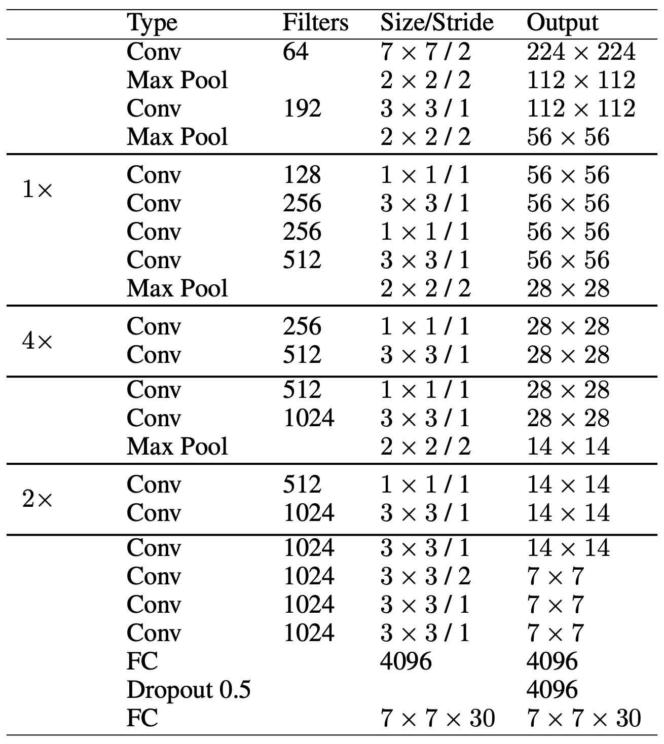
The architecture of YOLO v1 is a simple convolutional network with Maxpool layers and LeakyReLU activation functions followed by a linear layer and the prediction tensor.
To improve the speed of the network, they alternated convolutional layers with 3x3 kernel size and convolutional layers with 1x1 kernel size.
Here is why this speeds up the computation.
Without 1 x 1 convolution: Let’s assume for example that within the network, we have a feature map of size 56 x 56 x 192 (this means that the previous convolutional layer has 192 filters) and we want to apply a convolution layer of 256 filters of kernel size 3 x 3. For each filter, we have
\(56 \times 56 \times 192 \times 3 \times 3 = 5,419,008 \text{ computations}\)For all the filters we have
\(5,419,008 \times 256 = \sim 1.4 \text{B computations}\)With 1 x 1 convolution: Instead, let’s apply a convolution layer of 128 filters of kernel size 1 x 1 first. This leads to
\(56 \times 56 \times 192 \times 128 = 77,070,336 \text{ computations}\)and the resulting feature map is of size 56 x 56 x 128. Now, let’s apply our convolution layer of 256 filters with kernel size 3 x 3. We obtain
\(56 \times 56 \times 128 \times 3 \times 3 \times 256= 924,844,032 \text{ computations}\)Adding to that the computation of the previous convolution layer, we have
\(77,070,336 +924,844,032=\sim 1\text{B computations}\)
Therefore applying a 1 x 1 convolution prior to the 3 x 3 convolution reduces the dimensionality of the tensors and saves ~ 0.4B computations.
The Loss function
Now that we know what we predict, we need to define a bit better the optimization problem. Surprisingly enough, all the prediction targets are optimized using the mean error square (MSE) loss function.
Minimizing the error for the box center positions:
\(L_{\text{position}}=\sum_{i \in \text{grid}}\sum_{j \in \text{boxes}}\mathbb{I}_{\{\text{if object in } i\}}\left[\left(x_{i} - \hat{x}_{i} \right)^2 + \left(y_{i} - \hat{y}_{i} \right)^2\right]\)We simply minimize the MSE for x and y for each box from the ground truth values when an object exists in the cell. Here 𝐈{condition} is the indicator function (𝐈{condition} = 1 if condition and 0 otherwise).
Minimizing the error for the box shape:
\(L_{\text{shape}}=\sum_{i \in \text{grid}}\sum_{j \in \text{boxes}}\mathbb{I}_{\{\text{if object in } i\}}\left[\left(\sqrt{w_{i}}- \sqrt{\hat{w}_{i}} \right)^2 + \left(\sqrt{h_{i}} - \sqrt{\hat{h}_{i}} \right)^2\right]\)We minimize the square-root values of w and h for each box from the ground truth when an object exists in the cell. This is done to give more balance to smaller boxes during training.
Minimizing the error for the objectness:
\(L_{\text{objectness}}=\sum_{i \in \text{grid}}\sum_{j \in \text{boxes}}\mathbb{I}_{\{\text{if object in } i\}}a\left(1-\hat{C}_i\right)^2 + \mathbb{I}_{\{\text{if object not in } i\}}b\hat{C}_i^2 \)The weights a and b are different (a = 5 and b = 0.5) depending if there is an object or not in the cell because there are way more cells without objects than there are. This avoids biasing the model into overly predicting small values.
Minimizing the error for the predicted classes:
\(L_{\text{classes}} =\sum_{i \in \text{grid}}\mathbb{I}_{\{\text{if object in } i\}}\sum_{c\in \text{classes}}\left( p_i(c) - \hat{p}_i(c)\right)^2\)We minimize the MSE for p(c) for each class from the ground truth values when an object exists in the cell.
The overall loss function is simply the weighted sum of all the above losses:
The training
The network is pre-trained on the ImageNet data to learn the typical image features, and it is then fine-tuned on the PASCAL Visual Object Classes (VOC) 2007 and the VOC 2012 datasets. They used images with 448 x 448 resolution and image augmentations such as random scaling, translation, exposure, and saturation.
Non-maximum suppression
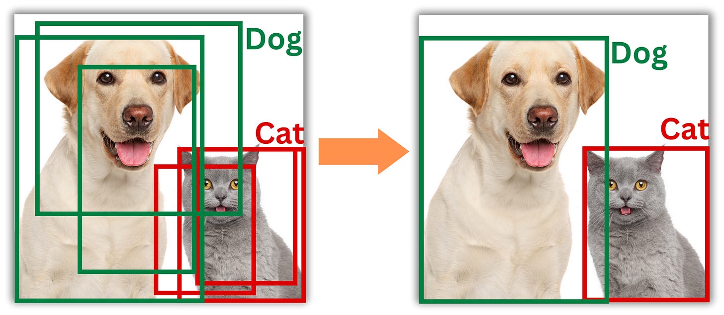
The process can lead to multiple bounding boxes being predicted for the same object. In such a case, we need to find a way to remove the redundant ones. The typical technique used is the so-called Non-maximum suppression
We first need to find all the boxes that overlap. The typical measure of overlap is Intersection over Union (IoU)


