Deep Neural Networks: All the Building Blocks
Do you have the mind of an Architect?
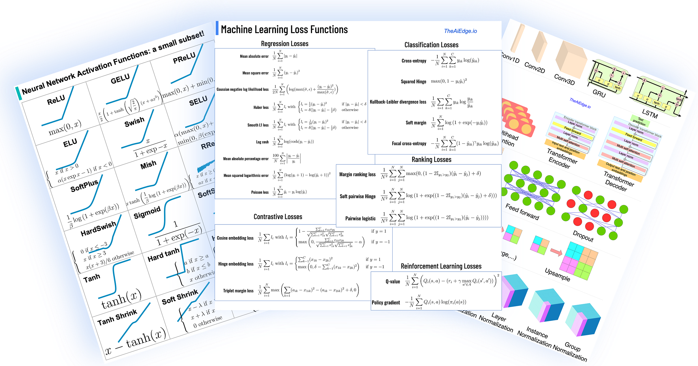
Today we dig deeper into the fastest-growing field of Machine Learning: Deep Learning. Deep Learning requires a more architect-like mindset than traditional Machine Learning. Smart rearrangements of the simple units presented here led to the discoveries of new capabilities of AI models not thought possible before that. We are going to look at:
The computational units
The Loss functions
The Activation functions
The computational units
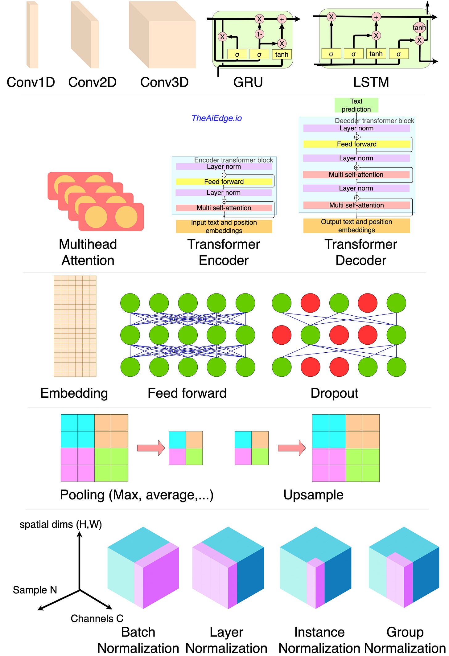
Deep Learning requires much more of an ARCHITECT mindset than traditional Machine Learning. In a sense, part of the feature engineering work has been moved to the design of very specialized computational blocks using smaller units (LSTM, Convolutional, embedding, Fully connected, …). I would always advise to start with a simple net when architecting a model such that you can build your intuition. Jumping right away into a Transformer model may not be the best way to start.
Most of the advancements in Machine Learning for the past 10 years come from a smart rearrangement of the simple units presented here. Obviously, I am omitting activation functions and some others here but you get the idea.
A convolutional layer is meant to learn local correlations. Multiple successive blocks of conv and pooling layers allows one to learn the correlations at multiple scales and they can be used on image data (conv2d), text data (text is just a time series of categorical variables) or time series (conv1d). You can encode text data using an embedding followed by a couple of conv1d layers. And you can encode a time series using a series of conv1d and pooling layers.
I advise against using LSTM layers when possible. The iterative computation doesn’t allow for good parallelism leading to very slow training (even with the Cuda LSTM). For text and time series ConvNet are much faster to train as they make use of the matrix computation parallelism and tend to perform on par with LSTM networks (http://www.iro.umontreal.ca/~lisa/pointeurs/handbook-convo.pdf). One reason transformers became the leading block unit for text learning tasks, is its superior parallelism capability compared to LSTM allowing for realistically much bigger training data sets.
Here are a couple of dates to understand the DL timeline:
(1989) Convolution layer and average pooling: “Handwritten Digit Recognition with a Back-Propagation”.
(1997) LSTM layer: “LONG SHORT-TERM MEMORY”
(2003) Embedding layer: “Quick Training of Probabilistic Neural Nets by Importance Sampling“.
(2007) Max Pooling: “Sparse Feature Learning for Deep Belief Networks“.
(2012) Feature dropout: “Improving neural networks by preventing co-adaptation of feature detectors“.
(2012) Transfer learning: “Deep Learning of Representations for Unsupervised and Transfer Learning“.
(2013) Word2Vec Embedding: “Efficient Estimation of Word Representations in Vector Space“.
(2013) Maxout network: “Maxout Networks“.
(2014) GRU layer: “On the Properties of Neural Machine Translation: Encoder–Decoder Approaches“.
(2014) Dropout layers: “Dropout: A Simple Way to Prevent Neural Networks from Overfitting“.
(2014) GloVe Embedding: “GloVe: Global Vectors for Word Representation“.
(2015) Batch normalization: “Batch Normalization: Accelerating Deep Network Training b y Reducing Internal Covariate Shift“.
(2016) Layer normalization: “Layer Normalization“.
(2016) Instance Normalization: “Instance Normalization: The Missing Ingredient for Fast Stylization“.
(2017) Self Attention layer and transformers: “Attention Is All You Need“.
(2018) Group Normalization: “Group Normalization“.
The Loss functions
Your Machine Learning model LOSS is your GAIN! At least if you choose the right one! Unfortunately, there are even more loss functions available than redundant articles about ChatGPT.
When it comes to regression problems, the Huber and Smooth L1 losses are the best of both worlds between MSE and MAE being differentiable at 0 and limiting the weight of outliers for large values. The LogCosh has the same advantage, having a similar shape to the Huber one. The mean absolute percentage error and the mean squared logarithmic error greatly mitigate the effects of outliers. Poisson regression is widely used for count targets that can only be positive.
For classification problems, cross-entropy loss tends to be king. I find the focal cross-entropy to be quite interesting, as it gives more weight to the samples where the model is less confident giving more focus on the "hard" samples to classify. The KL divergence is another information theoretic metric and I would assume it is less stable than cross-entropy in small batches due to the more fluctuating averages of the logs. The hinge loss is the original loss of the SVM algorithm. The squared hinge is simply the square of the hinge loss and the soft margin is simply a softer differentiable version of it.
Ranking losses tend to be extensions of the pointwise ones, penalizing the losses when 2 samples are misaligned compared to the ground truth. The margin ranking, the soft pairwise hinge and the pairwise logistic losses are extensions of the hinge losses. However, ranking loss functions are painfully slow to compute as the time complexity is O(N^2) where N is the number of samples within a batch.
Contrastive learning is a very simple way to learn aligned semantic representations of multimodal data. For example, triplet margin loss was used in Facenet (https://arxiv.org/pdf/1503.03832.pdf) and cosine embedding loss in CLIP (https://arxiv.org/pdf/2103.00020.pdf). The hinge embedding loss is similar but we replace the cosine similarity with the Euclidean distance.
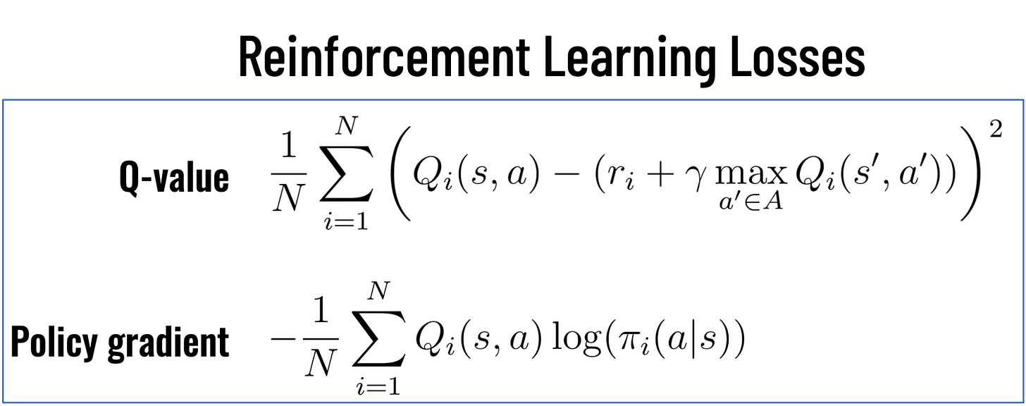
Deep Learning had a profound effect on Reinforcement Learning, allowing us to train models with high state and action dimensionalities. For Q-learning, the loss can simply take the form of the MSE for the residuals of the Bellman equation. In the case of Policy gradient, the loss is the cross-entropy of the action probabilities weighted by the Q-value.
And those are just a small subset of what exists. To get a sense of what is out there, a simple approach is to take a look at the PyTorch and TensorFlow documentation. These lecture notes are worth a read: “A Comprehensive Survey of Loss Functions in Machine Learning“.
The Activation functions
If you are looking for the "best" ACTIVATION function, be ready to spend some time looking for it because there are hundreds of them! Fortunately, you can safely cross-validate just a couple of them to find the right one. There are a few classes of activation functions (AF) to look out for:
The Sigmoid and Tanh based - Those activation functions were widely used prior to ReLU. People were very comfortable with those as they were reminiscent of Logistic Regression and they are differentiable. The problem with those is that, being squeezed between [0, 1] or [-1, 1], we had a hard time training deep networks as the gradient tends to vanish.
Rectified Linear Unit (ReLU) back in 2011 changed the game when it comes to activation functions. I believe it became very fashionable after AlexNet won the ImageNet competition in 2012. We could train deeper models but the gradient would still die for negative numbers due to the zeroing in x < 0. Numerous AF were created to address this problem such as LeakyReLU and PReLU.
Exponential AF such as ELU sped up learning by bringing the normal gradient closer to the unit natural gradient because of a reduced bias shift effect. They were solving for the vanishing gradient problem as well.
More recent activation functions use learnable parameters such as Swish and Mish. Those adaptive activation functions allow for different neurons to learn different activation functions for richer learning while adding parametric complexity to the networks.
The class of Gated Linear Unit (GLU) has been studied quite a bit in NLP architectures and they control what information is passed up to the following layer using gates similar to the ones found in LSTMs. For example Google's PaLM model is trained with a SwiGLU activation.
Here is a nice review of many activation functions with some experimental comparisons: “Activation Functions in Deep Learning: A Comprehensive Survey and Benchmark“. Looking at the PyTorch API and the TensorFlow API can also give a good sense of what are the commonly used ones.


