How Generative Adversarial Networks work!

Advanced Machine Learning

---

Generative Adversarial Networks (GANs) marked the first great success of Deep Learning when it comes to generative AI. We are reviewing the in and out of this foundational model paradigm. We are going to look at:

• The overview of GAN’s architecture

• The discriminator

• The generator

• The training

• The loss functions

• The convergence of the generative training

---

Overview of GAN’s architecture

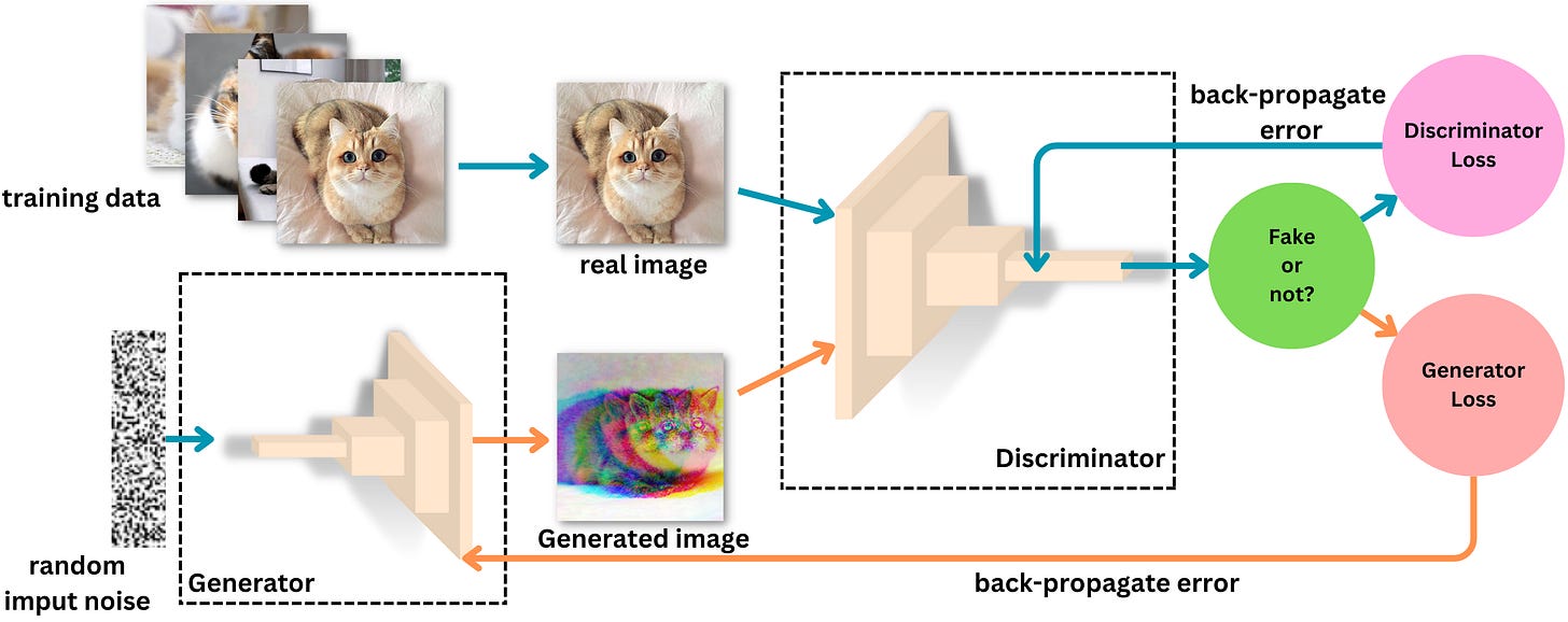
The goal of Generative Adversarial Networks (GANs) is to generate fake images that seem realistic. GANs can be broken down into the following components:

• The generator - The role of the generator is to fool the discriminator into generating images as realistic as possible

• The discriminator - the role of the discriminator is to distinguish the generated images from the real ones

• The loss functions - The loss functions are there to capture the problem as an optimization problem and will allow the model to learn. The discriminator wants to become very good at distinguishing real images from fake ones and the generator wants to become very good at fooling the discriminator with fake images.

The Discriminator

The discriminator is simply a classifier. The input data are real images and generated images and the labels are “1“s if the image is real and “0“ if not.

In the 2014 original paper by Ian J. Goodfellow (“Generative Adversarial Nets“), the proposed discriminator was simply a feedforward network. In 2016 Alec Radford and Luke Metz proposed DCGAN, a convolutional network architecture (“Unsupervised Representation Learning with Deep Convolutional Generative Adversarial Networks”) with a discriminator architecture very close to the VGG16 architecture (“Very Deep Convolutional Networks for Large-Scale Image Recognition”). The architecture is comprised of a succession of convolutional layers where, for each layer, the number of output channels is twice as big as the number of input channels. The final computational unit is a sigmoid for binary classification (fake or not):

The following pseudo-code captures the architecture of the discriminator:

discriminator = Sequential(
    # first layer
    Conv2d(3, 64),
    LeakyReLU(0.2),

    # second layer
    Conv2d(64, 128),
    BatchNorm2d(),
    LeakyReLU(0.2),

    # third layer
    Conv2d(128, 256),
    BatchNorm2d,
    LeakyReLU(0.2),
    
    # fourth layer
    Conv2d(256, 512),
    BatchNorm2d,
    LeakyReLU(),
    
    # fifth layer
    nn.Conv2d(512, 1),
    Sigmoid()
)

The Generator

The generator takes as input random noise and outputs an image. Its architecture is very similar to that of the discriminator, but performs the opposite operation:

Figure 1 of “Unsupervised Representation Learning with Deep Convolutional Generative Adversarial Networks”

The main difference is that instead of using convolution operations, the generator uses transposed convolution operators. They can be seen as estimators of inverse convolution operations:

Transposed convolution with half padding, no strides. Source: https://github.com/vdumoulin/conv_arithmetic/blob/master/README.md

The following pseudo-code captures the architecture of the generator:

generator = Sequential(
    # first layer
    ConvTranspose2d( 100, 512),
    BatchNorm2d,
    ReLU,
    # second layer
    ConvTranspose2d(512, 256),
    BatchNorm2d,
    ReLU,
    # third layer
    ConvTranspose2d(256, 128),
    BatchNorm2d,
    ReLU,
    # forth layer
    ConvTranspose2d(128, 64),
    BatchNorm2d,
    ReLU,
    # fifth layer
    ConvTranspose2d(64, 3),
    Tanh()
)

The Training

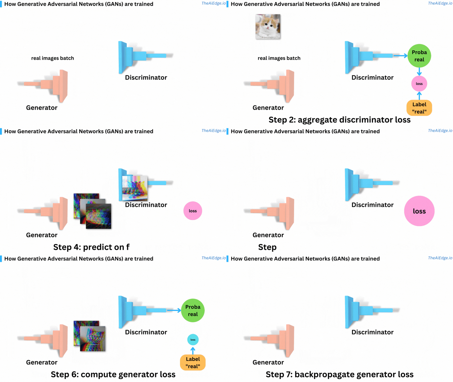
Training a GAN can be tricky. We iterate over epochs and data batches. The data needs to represent the distribution of images you are trying to learn. Here are the steps for one batch of images within an epoch:

• Step 1 - We get the predictions from the discriminator on the data batch. The discriminator is trying to estimate the probability that the sample is real.