How to Optimize LLM Pipelines with TextGrad

When we build Large Language Model applications, we likely have to pipe multiple LLM calls before getting an answer. Each LLM call has its own system prompt and user prompt, and if one call yields suboptimal results, the whole pipeline will suffer from it. Let’s consider the following RAG pipeline example:

To ensure the quality of the responses generated by the pipeline, we usually need multiple LLM calls before the answer can be returned:

• Routing the question: it can be a good practice to implement a routing system that routes the question to the RAG system only if the question requires additional context to be answered.

• Preprocessing the question: it is often better to reframe the user question into a text query that may retrieve more relevant documents for answering the question.

• Answering the question with the database context: Once we have retrieved the data, we can include it as context in the prompt to answer the question.

• Validating the response: it can be good practice to validate that the response is actually relevant to the question before sending it to the user and have a fallback mechanism in place in case the generated response is not satisfactory.

It is possible to build very robust pipelines by implementing routing, check, validation, and fallback nodes at the expense of higher latency. Each node requires its own system prompt, and tuning them correctly can be a challenge as the change in one prompt will influence the inputs into the other ones. With large pipelines, we run the risk of accumulating errors from one node to the next, and it can become tough to scale the pipeline beyond a few nodes.

A new strategy that has silently been revolutionizing the field of orchestrated LLM applications is LLM pipeline optimization with optimizers. DSPy has established the practical foundation of the field, and new techniques like TextGrad and OPRO have emerged since then. Let’s study the ideas behind TextGrad in a simple example.

The Backpropagation Algorithm in Neural Networks

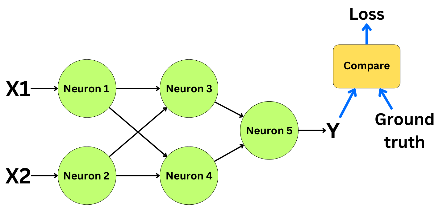
The idea behind TextGrad is to optimize pipelines with an approach similar to the backpropagation algorithm. The backpropagation is the algorithm used to train neural networks. Let’s consider this simple neural network, for example, where we have two input features, X1 and X2, and a prediction Y:

Constructing the graph

There are a few features necessary to build a backpropagation-like algorithm. We need a way to capture the graph structure of the neural network. Each neuron needs to know where its information is coming from to be able to correctly backpropagate the error during the backward pass. Constructing the graph structure is done during the forward pass of the backpropagation algorithm:

Measuring a loss function

We then need a way to measure how good or bad the current prediction is. That is the role of the loss function! We compare the prediction of the model to the ground truth value of the training data.

For example, for regression tasks, we typically use the mean square error loss, and for classification tasks, we use the cross-entropy loss function:

The loss function should be constructed such that it exists an analytical form of the gradient of the function with respect to the predictions:

\(\mathrm{Gradient\ of\ the\ Loss}=\nabla_{\hat{y}}\mathrm{Loss}\)

The function should have its minimal value when the predictions are perfect and should be large when the predictions are bad.

Improving the network

The loss function will tell us how we should modify the model parameters to get better predictions. Because we want to minimize the loss function, we want to modify the model parameters such that it decreases the loss function. This is the foundation for the gradient descent algorithm:

\(\theta_t = \theta_{t-1} - \alpha\nabla_{\theta}\mathrm{Loss}\)

The gradient of the loss with respect to the model parameters can be derived with the chain rule from the gradient with respect to the predictions:

\(\nabla_{\theta}\mathrm{Loss}=\nabla_{\hat{y}}\mathrm{Loss}\nabla_{\theta}\hat{y}\)

This is important to understand what those quantities are telling us:

The optimization step is just an improvement of the model parameters based on that feedback:

\(\theta_t = \theta_{t-1} - \alpha\nabla_{\theta}\mathrm{Loss}\)

Backpropagating the gradients

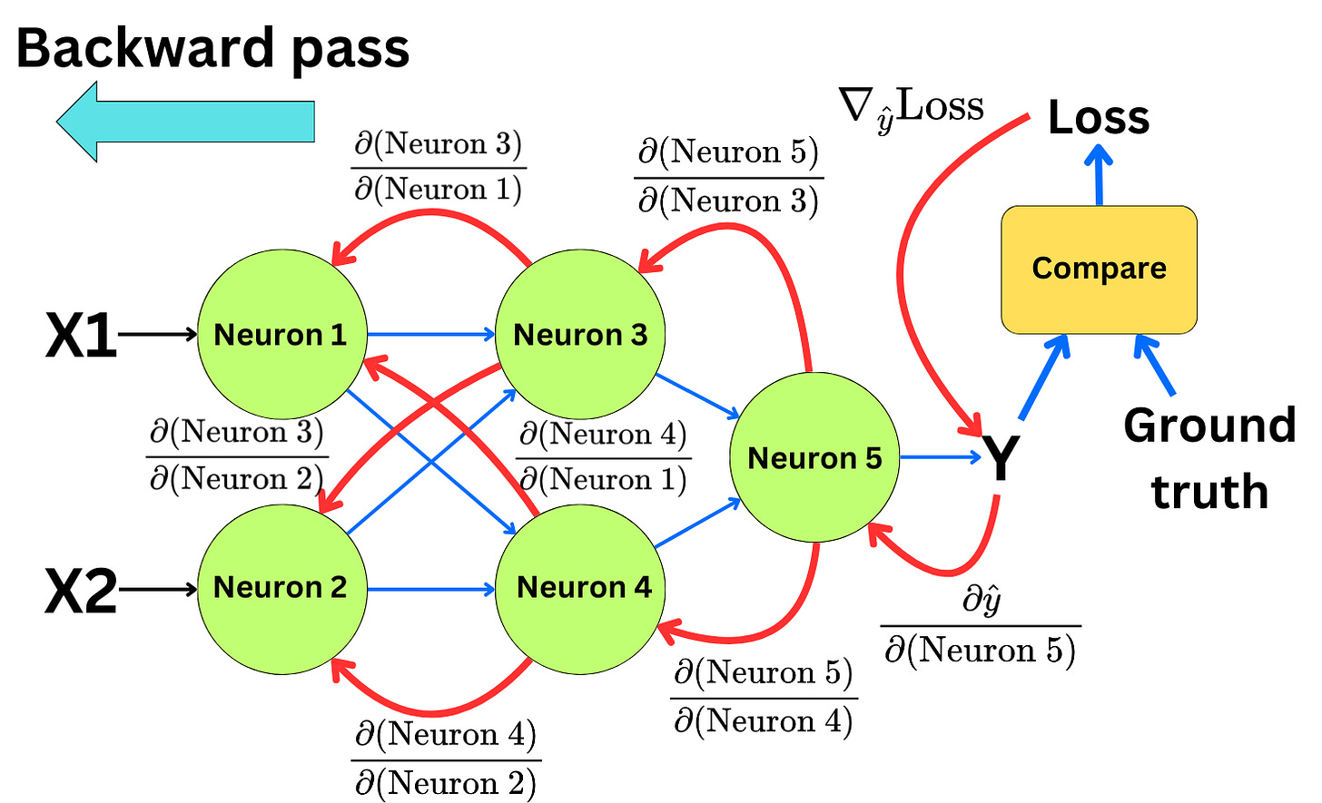
To be able to apply the gradient descent optimization step to all the parameters in the network we need to backpropagate the gradients to each neuron in the network. This is done with the chain rule. If we know the gradient of the loss in layer n, we can derive the gradient of the loss in layer n-1:

\(\nabla_{\mathrm{layer\ }n-1}\mathrm{Loss}=\nabla_{\mathrm{layer\ }n-1}(\mathrm{layer\ }n)\nabla_{\mathrm{layer\ }n}\mathrm{Loss}\)

With the chain rule, we can iterate from the end of the network to the beginning of it and compute the gradient of the loss function for every parameter in the network:

This is what we call the backward pass.