Mixture-of-Experts: Early Sparse MoE Prototypes in LLMs

Mixture-of-Experts might be one of the most important improvements in the Transformer architecture! It allows for scaling the number of model parameters while keeping the latency associated with the forward and backward pass of the backpropagation algorithm almost constant. Scaling in the width direction, as opposed to the depth of the model, allows for keeping the gradient paths short, improving the stability of the training. We explore here 2 early models:

• The Sparsely-Gated Mixture-of-Experts Layer

• GShard

---

The First Mixture-of-Experts

The concept of the Mixture of Experts (MoE) architecture was introduced in 1991 by Jacobs et al. The idea was to combine the learning of parallel learners using a gating mechanism. The goal was to increase the model's capacity while maintaining stable training and achieving faster convergence. Deep networks tend to suffer from vanishing or exploding gradients, and extending the capacity in the width direction allows for the learning of more complex statistical patterns while keeping short gradient paths.

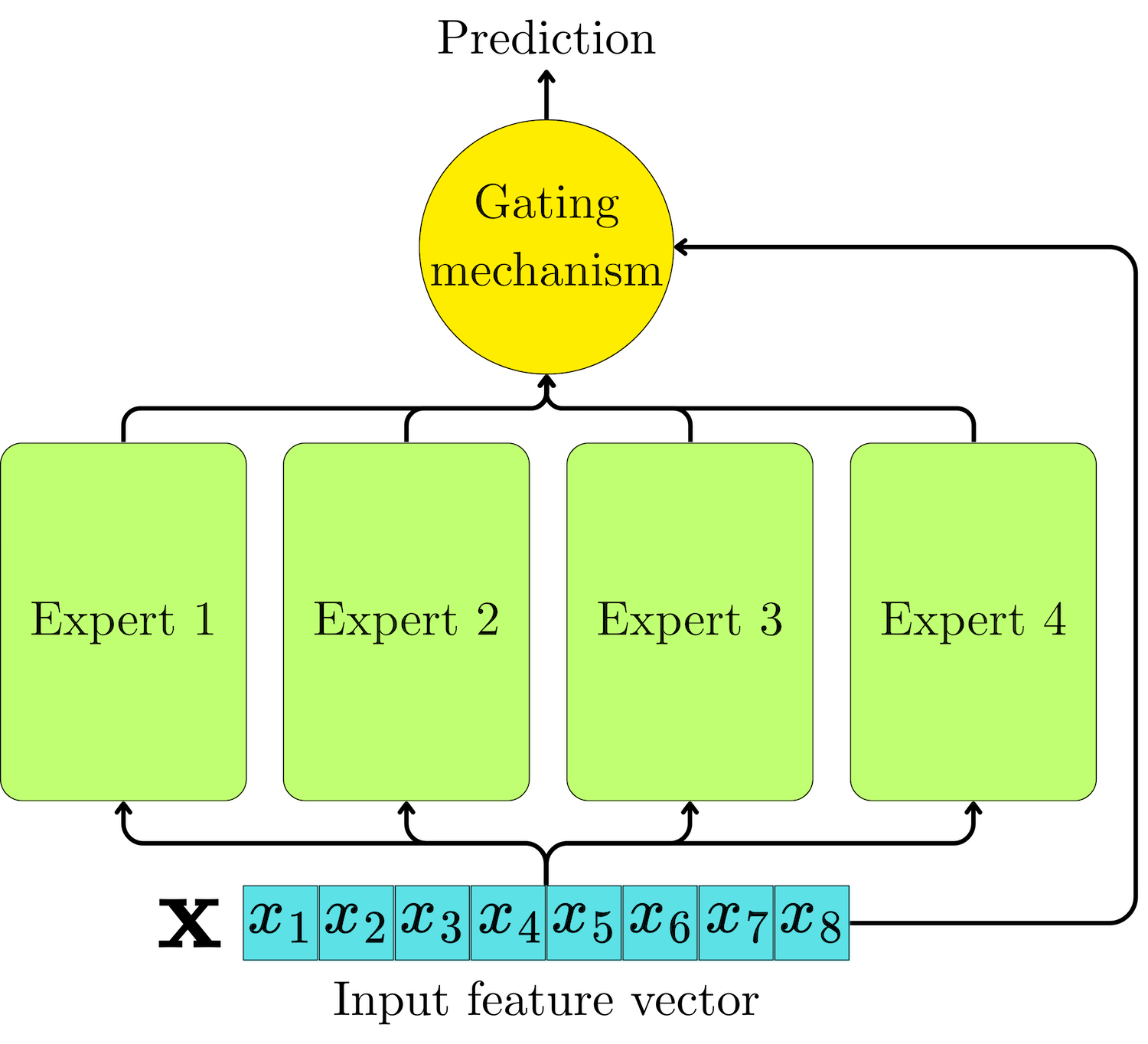
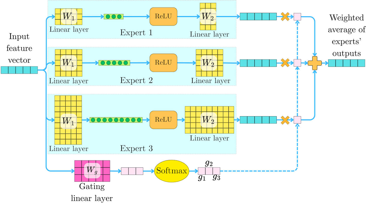
An "expert" E_i can be a simple feed-forward network. For example:

\(E_i(\mathbf{h})= \text{ReLU}\left(W_1^i\mathbf{h} + \mathbf{b}_1\right)W_2^i + \mathbf{b}_2\)

where W₁ⁱ and W₂ⁱ may have different dimensions depending on the expert. The gating mechanism generates a weight g_i(h) for each expert, and the MoE output is a weighted average of the experts' outputs:

\( \mathbf{y} = \sum_{i=1}^n g_i(\mathbf{h})E_i(\mathbf{h})\)

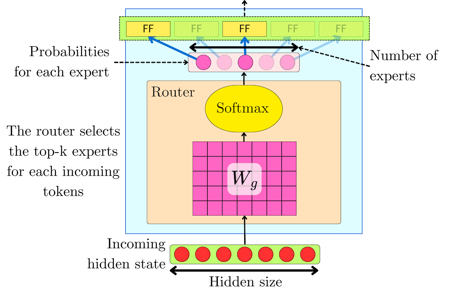
g_i(h) is typically the softmax transformation of a linear projection W_g of the input features:

\(\mathbf{g}(\mathbf{h}) = \text{Softmax}\left(W_g\mathbf{h} + \mathbf{b}_g\right)\)

where W_g is a linear layer of dimension |h| ⨉ n. The softmax transformation yields a probability-like value that captures the proportion of contributions for each expert.

Early Sparse MoE Prototypes in LLMs

The Sparsely-Gated Mixture-of-Experts Layer

The Sparse mechanism

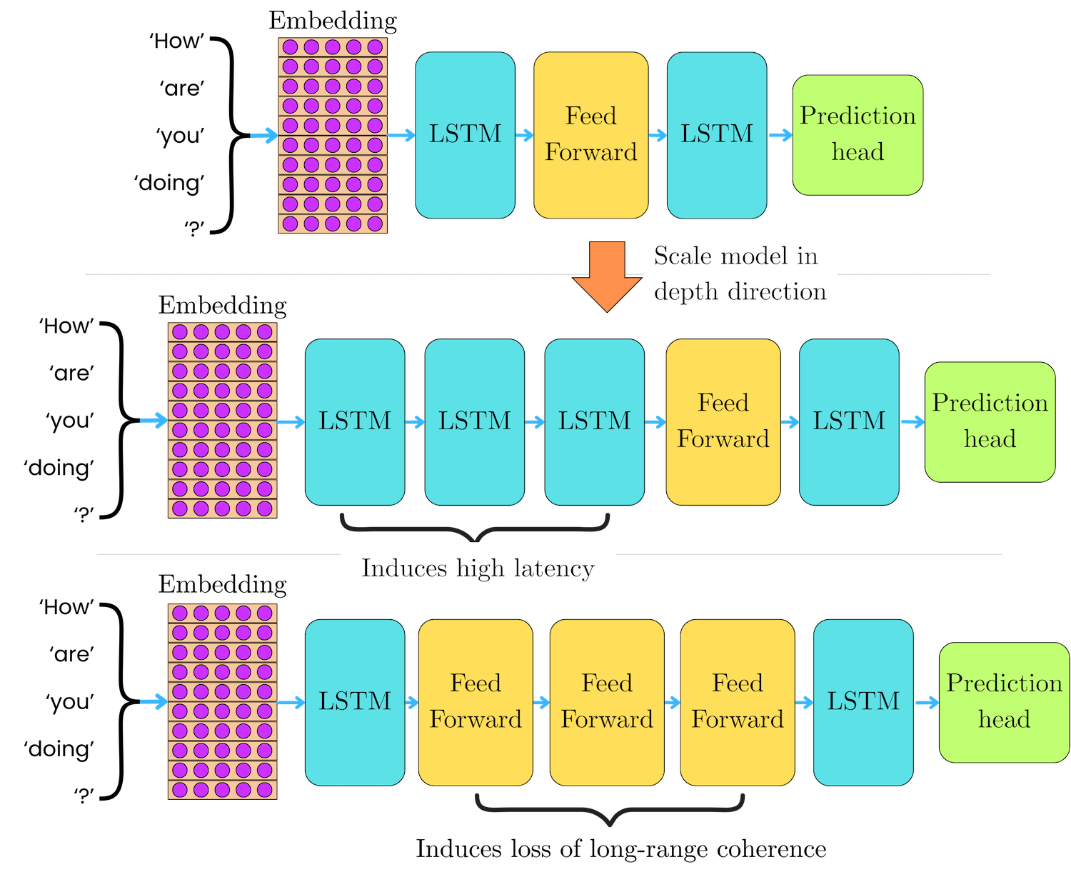
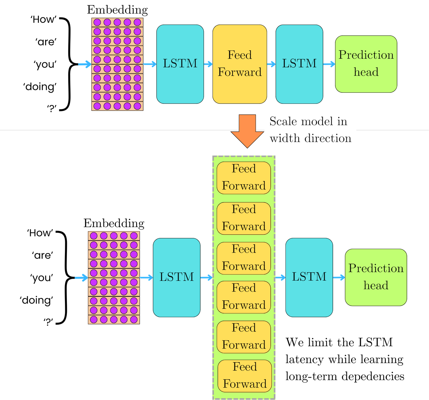
The sparse Mixture of Experts (MoE) architecture was introduced by Shazeer et al in January 2017 in LSTM-based language models as a way to drastically scale the model capacity while keeping the number of operations constant, independent of the number of experts. RNN models are hard to scale because the LSTM operations are intrinsically iterative, preventing the high parallelism provided by other computational units. Scaling in depth with more LSTM units induces high latency, while scaling with feed-forward networks limits the ability of the LSTM layers to capture long-range coherence of the input sequences. Scaling in width with many parallel experts permits the LSTM to learn the long-term dependencies while keeping the latency to a minimum.

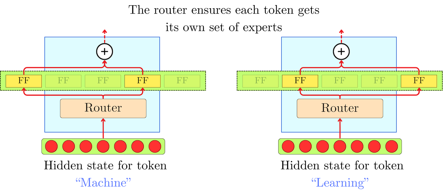
To keep the number of operations independent of the number of experts, they introduced a routing mechanism that selects the top-k experts for each token. They tested a total number of experts that ranged between 4 and 131,072, but only the top-4 experts were used for each token.

For the sparse MoE, the architecture is the same for every expert i:

\(E_i(\mathbf{h})= \text{ReLU}\left(W_1^i\mathbf{h} + \mathbf{b}_1\right)W_2^i + \mathbf{b}_2\)

The gating mechanism is, as before, induced by a linear layer W_g mapping from hidden size d_model to n with an added normal noise ϵ:

\(\mathbf{l}(\mathbf{h}) = W_g \mathbf{h} + \epsilon\)

The noise allows the model to uniformly explore the different experts in the early part of the training and prevents the collapse onto a handful of "favorite" experts. To generate the noise, the input vector is first projected with another linear layer W_n passed through a softplus transformation:

\(\sigma(\mathbf{h}) = \text{Softplus}(W_n \mathbf{h}) = \log(1 + \exp(W_n \mathbf{h})) \)

The resulting value 𝛔(h) is used as the standard deviation to generate the normal noise:

\(\epsilon \sim \mathcal{N}(0, \sigma(\mathbf{h}))\)

The standard deviation 𝛔(h) controls how much randomness is injected for each expert on that particular input token. Larger 𝛔(h) will lead to more exploration, and smaller 𝛔(h) will push the gate to behave almost deterministically. Softplus is basically a "soft" version of ReLU: for large positive values, it increases linearly and flattens near 0. It is used here to make sure the learned noise scale 𝛔(h) is positive and differentiable everywhere. Because the noise is input‑adaptive, the router can start off as a near‑uniform sampler (large 𝛔(h)) and gradually anneal into a confident switch (small 𝛔(h)).

Once the logits l(x) = {l₁(h), l₂(h), …, l_n(h)} have been computed, we mask the non-top-k's contribution with -∞:

\(\overline{l}_i(\mathbf{h})= \begin{cases} l_i(\mathbf{h}), & \text{if } l_i(\mathbf{h})\text{ is in the top-}k,\\ -\infty, & \text{otherwise}. \end{cases}\)

And we perform a softmax transformation to obtain the contribution of each top-k expert:

\(\mathbf{g}(\mathbf{h}) = \frac{e^{\overline{\mathbf{l}}(\mathbf{h})}}{\sum_{i=1}^n e^{\overline{l}_i(\mathbf{h})}}\)

The -∞ masks will lead to g_i(h) = 0 contribution for every non-top-k expert while keeping the softmax normalization as if only the top-k experts contributed to the sum. The resulting hidden state y(h) is the weighted average of top-k experts' output:

\( \mathbf{y}(\mathbf{h})=\sum_{i\in \text{top-}k} g_i(\mathbf{h})E_i(\mathbf{h})\)

Hierarchical Mixture of Experts

In the Sparsely-Gated Mixture-of-Experts, they scaled the number of experts up to 131,072! With naive MoE, the gate and noise projection layers W_g and W_n would require a dimension (n ⨉ d_model) ~ 67M parameters (with d_model = 512), with as many operations for each token in the input sequence. At this scale, the gating mechanism becomes the bottleneck. Instead, they introduced a hierarchical gating process where the experts were grouped into a blocks of b experts. The first gate projects from d_model to a blocks:

\(\mathbf{l}^{(1)}(\mathbf{h}) = W_g^{(1)} \mathbf{h} + \epsilon^{(1)}\)

From this first set of logits, we can pick the top-k₁ expert blocks: