Understanding How Vector Databases Work!

May 02, 2024

The rise of Vector databases

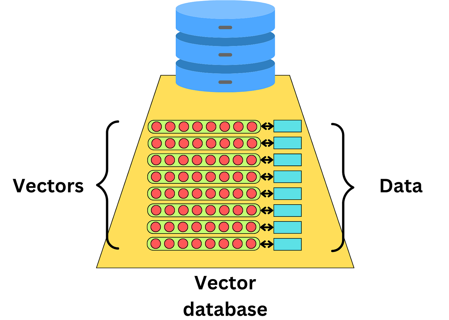
We have recently seen a surge in vector databases in this era of generative AI. The idea behind vector databases is to index the data with vectors that relate to that data

Vector databases are often used for recommender engines where we learn vector representations of users and items we want to recommend

This allows one to quickly find similar items by using an approximate nearest-neighbor search

As long as we can learn a vector representation of a piece of data, we can index it in a vector database. With the recent advent of LLMs, it became easier to compute vector representations of text documents, capturing the semantic meaning of that text

Vector databases make it easier to find semantically similar text documents

Different vector databases

There are tons of vector database providers. Here is a small list of such databases:

Pinecone: A vector database that is designed for machine learning applications. It supports a variety of machine learning algorithms and is built on top of Faiss, an open source library by Meta for efficient similarity search of dense vectors.
Deep Lake: Deep Lake is a Database for AI powered by a unique storage format optimized for deep-learning and Large Language Model (LLM) based applications. It simplifies the deployment of enterprise-grade LLM-based products by offering storage for all data types (embeddings, audio, text, videos, images, pdfs, annotations, etc.), querying and vector search, data streaming while training models at scale, data versioning and lineage for all workloads, and integrations with popular tools such as LangChain, LlamaIndex, Weights & Biases, and many more.
Milvus: Milvus is an open-source vector database built to power embedding similarity search and AI applications. Milvus makes unstructured data search more accessible and provides a consistent user experience regardless of the deployment environment.
Qdrant: is a vector similarity search engine and vector database. It provides a production-ready service with a convenient API to store, search, and manage points—vectors with an additional payload Qdrant is tailored to extended filtering support. It makes it useful for all sorts of neural network or semantic-based matching, faceted search, and other applications.
Weaviate: Weaviate is an open-source vector database that is robust, scalable, cloud-native, and fast. With Weaviate, you can turn your text, images, and more into a searchable vector database using state-of-the-art ML models.

These are just a small sample of the available vector databases. I found that looking at LangChain vectorstore integration documentation provides a wider list of available vector databases.

Indexing and searching a vector space

Indexing a vector database is very different from indexing most databases. The goal of a query is to return the nearest neighbors as measured by a similarity metric. The typical time complexity for the K-nearest neighbor algorithm is O(ND), where N is the number of vectors and D is the vector dimension. The time complexity scales with the number of items which makes it unmanageable to build a scalable and fast database. The typical approach is to rely on Approximate Nearest Neighbor algorithms (ANN) to make the search blasting fast.

We here go over 3 different algorithms used for vector search: Product Quantization, Locality-sensitive hashing and Hierarchical Navigable Small World. Those are typical algorithms used in most vector databases. They are likely to be used in a combined manner for optimal retrieval speed.

Product Quantization

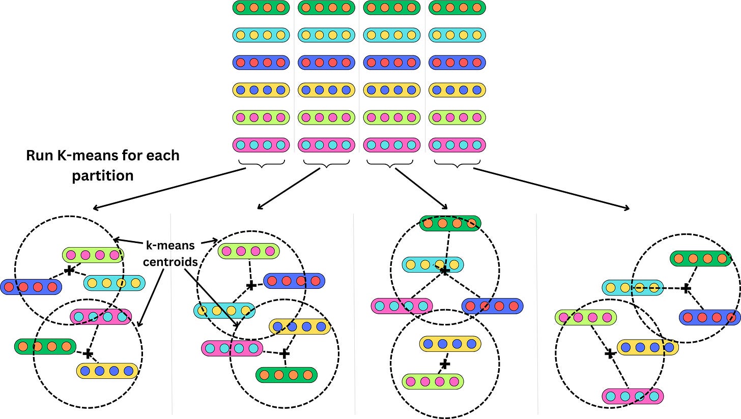
When looking for the nearest neighbors, it is often not important to be perfectly accurate. Product Quantization (PQ) is a way to quantize the vector space to represent vectors with less precision. The idea is to cluster vectors and index the cluster centroids instead of the vectors themselves. When looking for the nearest neighbors to a query vector, we just need to pull the vectors from the closest cluster. It is a faster search, and indexing the vectors takes much less memory space.

We first need to partition each vector into smaller vectors

and run a k-means algorithm on each partition

Instead of indexing the vectors, we index the centroid of the clusters they belong to. If we use 2 clusters per partition and have 6 vectors, that's 3X data compression. Obviously, the compression would be much higher with more vectors. Each vector now maps to a set of clusters and their related centroids.

If we want to find the nearest neighbors from a query vector, we measure the squared Euclidean distance for each cluster in each partition and return the vectors with the lowest summed squared Euclidean distances

Instead of having to iterate through each vector, we just need to iterate through the clusters’ centroids. There is a balance between search latency and accuracy. The more clusters we use, the better will be the hash and more accurate will be the returned nearest neighbors, but it will increase the search latency as we will need to iterate through more clusters.

This is still a brute-force approach as the algorithm scales with the number of clusters, but it can be used in combination with other algorithms.

Locality-sensitive hashing

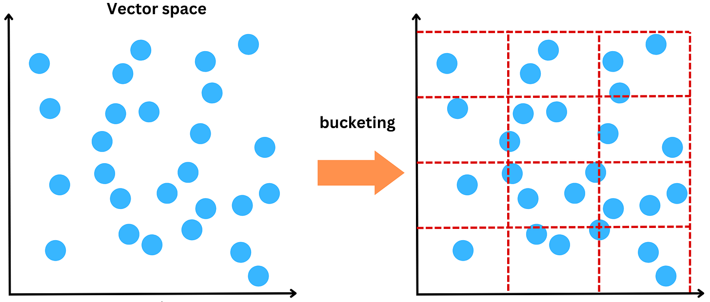
Locality-sensitive hashing (LSH) aims to group vectors together based on similarity. For example, we could partition the vector space into multiple buckets

and we could call “nearest neighbors” whatever vectors belong to the same bucket

Hashing a vector

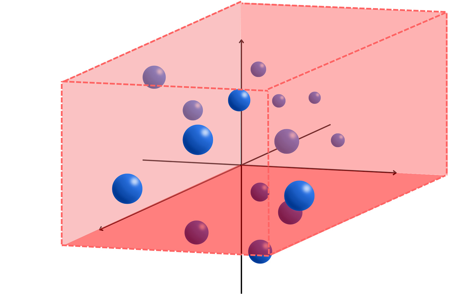
In practice, it is done a bit differently. An efficient way to partition the space is to project the vectors onto a space of a specific dimensionality and “binarize“ each component. The projection is done using a random matrix M of dimension (C, R) where C is the dimension of the original vector V and R is the dimension of the space we want to project the vectors into

\(V'=V\cdot M^T\)

For example, if C = 2 and R = 3, we would have something like that

We can now partition the space with regions above and below the hyperplanes at the origin

If we have for example, a vector A = [0.5, -1.5, 0.3], we look at each of the components and assign a 1 if it is positive and 0 otherwise

The vector A would be hashed to [1, 0, 1] under that process. Every vector assigned the same hash will be close in the vector space and can be labeled “nearest neighbors”. The time complexity to hash a vector V is O(R x C + R) = O(R x C), and retrieving the vectors with the same hash can be done in constant time.

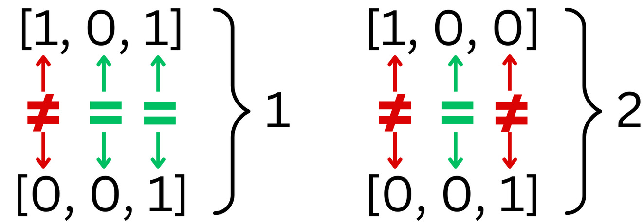
The distance between 2 vector’s hashes: Hamming Distance

The hash of a vector under the LSH hashing process is a binary vector. To measure how different 2 binary vectors are, we use the Hamming Distance. The Hamming distance counts the number of times 2 strings have different characters

When we have strings of binary numbers, the Hamming distance can be computed using the XOR operation and count the number of resulting 1s.

\(\begin{align*} 101 \oplus 001 = 100 \Rightarrow 1\\ 100 \oplus 001 = 101 \Rightarrow 2 \end{align*}\)

Hierarchical Navigable Small World

Hierarchical Navigable Small World (HNSW) is one of the most efficient ways to build indexes for vector databases. The idea is to build a similarity graph and traverse that graph to find the nodes that are the closest to a query vector.

Navigable Small World

Navigable Small World (NSW) networks is a process to build efficient graphs for search. Let’s imagine we have multiple vectors we need to index. We build a graph by adding them one after the other and connecting each new node to the most similar neighbors.

In the above example, we connected each new node to the 2 most similar neighbors, but we could have chosen another number of similar neighbors. When building the graph, we need to decide on a metric for similarity such that the search is optimized for the specific metric used to query items. Initially, when adding nodes, the density is low, and the edges will tend to capture nodes that are far apart in similarity. Little by little, the density increases, and the edges start to become shorter and shorter. As a consequence, the graph is composed of long edges that allow us to traverse long distances in the graph and short edges that capture closer neighbors. Because of it, we can quickly traverse the graph from one side to the other and look for nodes at a specific location in the vector space.

For example, let’s have a query vector. We want to find the nearest neighbor

We initiate the search by starting at one node (i.e. node A in that case). Among its neighbors (D, G, C), we look for the closest node to the query (D). We iterate over that process until there are no closer neighbors to the query. Once we cannot move anymore, we found a close neighbor to the query. The search is approximate and the found node may not be the closest as the algorithm may be stuck in a local minima.

Hierarchical graph

The problem with NSW is that we spend a lot of iterations traversing the graph to arrive at the right node. The idea for the Hierarchical Navigable Small World is to build multiple graph layers, with each layer being less dense than the next. Each layer represents the same vector space, but not all vectors are added to the graph. Basically, we include a node in the graph at layer L with a probability P(L). We include all the nodes in the final layer (if we have N layers, we have P(N) = 1), and the probability gets smaller as we get toward the first layers. We have a higher chance of including a node in the following layer, and we have P(L) < P(L + 1)

The first layer allows us to traverse longer distances at each iteration, whereas in the last layer, each iteration will tend to capture shorter distances. When we search for a node, we start first in layer 1 and go to the next layer if the NSW algorithm finds the closest neighbor in that layer. This allows us to find the approximate nearest neighbor in fewer iterations in average

It is not hard to extend this algorithm to multiple nearest neighbors.

Similarity Measures

When we query items in a vector database, we need to define what “similar vectors” means. There are plenty of metrics used to compute similarities between 2 vectors. Here, we dig into the most used similarity measures and how they differ from each other: Euclidean distance, dot product, and cosine similarity.

Euclidean distance

Let’s say we have a vector A = [a₁, a₂] and a vector B = [b₁, b₂], the Euclidean distance is simply

\(d(A, B) = \sqrt{\left(a_1-b_1\right)^2+\left(a_2-b_2\right)^2}\)

It measures how close are 2 points in a vector space. When a model learns a vector representation for a specific datum, the different components may capture vastly different information about the data, but Euclidean distance tends to completely ignore those

Dot product

With a vector A = [a₁, a₂] and a vector B = [b₁, b₂], the dot product is simply

\(\vec{A}\cdot \vec{B}=a_1b_1+a_2b_2\)

It can also be expressed as

\(\vec{A}\cdot\vec{B}=\Vert A\Vert\cdot\Vert B\Vert \cos \theta\)

Where ||A|| is the norm of the vector A and 𝜃 is the angle between A and B

This means that if 𝜃 > 90° then cos 𝜃 < 0. In the case 𝜃 = 180°, we have cos 𝜃 = -1 and

\(\vec{A}\cdot\vec{B}=-\Vert A\Vert\cdot\Vert B\Vert \)

So, depending on how the vectors are placed with respect to the origin, they may have the same exact Euclidean distances but opposite dot products

Cosine similarity

The Cosine similarity is a normalized dot product by the vectors’ magnitudes

\(S(A, B) = \frac{\vec{A}\cdot \vec{B}}{\Vert \vec{A}\Vert\cdot \Vert \vec{B}\Vert}\)

Because

\(\vec{A}\cdot\vec{B}=\Vert A\Vert\cdot\Vert B\Vert \cos \theta\)

we actually have

\(S(A, B) = \cos \theta\)

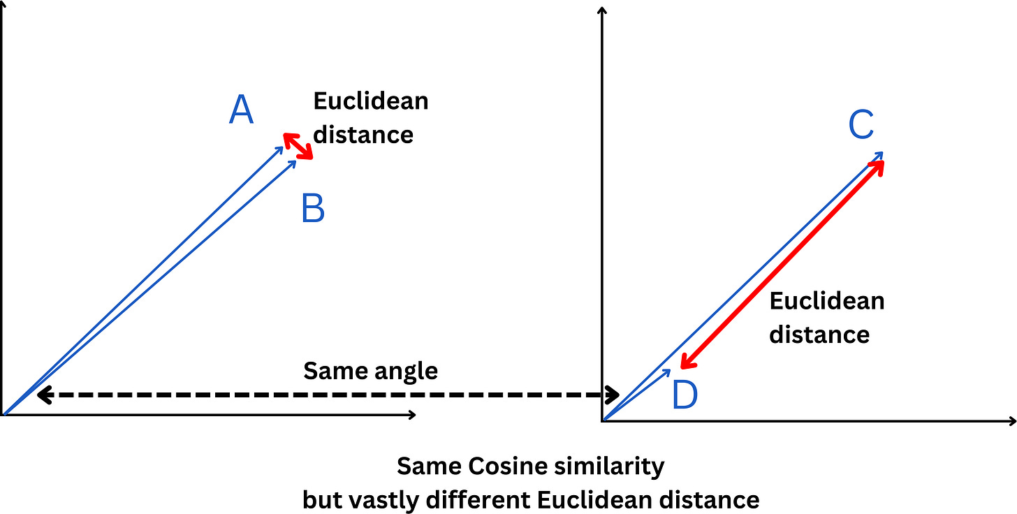
This means that 2 vectors will have the same cosine similarity independent of their magnitudes. For example, here the 2 sets of vectors have the same cosine similarity but vastly different Euclidean distance

Beyond indexing

Vector databases go beyond indexing and approximate nearest-neighbor search algorithms. Vector databases are specifically designed to manage vector embeddings and offer several advantages:

Database operations: As any database, we have the typical database operations such as insert, delete, and update operations.
Metadata and filtering: Vector databases allow the storage of metadata associated with each vector. This feature facilitates more precise queries, with users able to filter results based on additional metadata.
Scalability: Vector databases are built to scale according to increasing data volumes and support for distributed and parallel processing.