Understanding The Computational Graph in Neural Networks
Do you know what is this computational graph used by deep learning frameworks like TensorFlow or PyTorch? The whole logic behind how neural networks function is the back-propagation algorithm. This algorithm allows to update the weights of the network so that it can learn. The key aspect of this algorithm is to make sure we can compute the derivatives or the gradients of very complex functions. That is the whole point of the computational graph! It is to make sure we can backpropagate those derivatives to the whole network, no matter how deep it may be. So Let me show you how it works!
Watch the video for the full content!
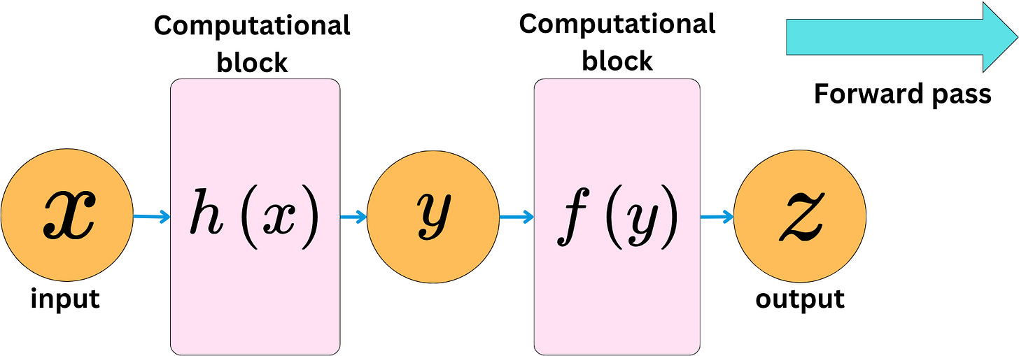
One important aspect of Deep Learning is the need to compute the derivatives of complex functions efficiently. In neural network frameworks like PyTorch, this is handled by storing the operations and variables of functions on a computational graph. Nodes represent the variables, and the edges represent operations. An incoming edge means a new variable has been created by applying an operation on other variables.
Creating the graph and computing the values at the different nodes is called the forward pass.
For each operation we apply, we know the derivative rules for the different variables involved, so we can easily compute the derivatives of the output variables as a function of the input variables. For a specific node, we only need to compute the derivatives of the outgoing variable with respect to the incoming variables. By applying the derivative chain rule, we can compute the derivatives of the output variables with respect to input variables for the whole graph. At every point of the process, we only compute the basic derivatives for a triplet of variables, but the chain rule allows us to compute derivatives for extremely complex functions.
Back-propagating the derivatives to the inputs of the graph is referred to as the backward pass.
We can easily implement this in PyTorch:
import torch

x = torch.tensor([2.0], requires_grad=True)
y = torch.tensor([3.0], requires_grad=True)
z = torch.tensor([4.0], requires_grad=True)

# Perform the operation
f = x * y * z  # f(x, y, z) = x * y * z

# Compute gradients
f.backward()

# Gradients: df/dx = y * z, df/dy = x * z, df/dz = x * y
print(f"Gradient df/dx: {x.grad}")  # Output should be 3.0 * 4.0
print(f"Gradient df/dy: {y.grad}")  # Output should be 2.0 * 4.0
print(f"Gradient df/dz: {z.grad}")  # Output should be 2.0 * 3.0

> Gradient df/dx: tensor([12.])
> Gradient df/dy: tensor([8.])
> Gradient df/dz: tensor([6.])
We can have complex computational blocks and still easily backpropagate the derivatives.
The chain rule always reduces the problem to a simple product operation. The backward pass computes the gradient of the output with respect to the inputs.
For example, in PyTorch:
def h(x):
    return x**2

def f(y):
    return y + 1


# Define tensors
x = torch.tensor(2.0, requires_grad=True)

# Define the computational blocks
y = h(x)  # Some function h
z = f(y)  # Some function f

# Compute gradients
z.backward()

# x.grad will contain ∇_{x}z
print("Gradient of z with respect to x:", x.grad)

> Gradient of z with respect to x: tensor(4.)
The network and the related functional relationship between the inputs and outputs can be as complex as we want.
Computing the derivatives (gradients) will always reduce to computing simple products due to the chain rule.
SPONSOR US
Get your product in front of more than 64,000 tech professionals.
Our newsletter puts your products and services directly in front of an audience that matters - tens of thousands of engineering leaders and senior engineers - who have influence over significant tech decisions and big purchases.
To ensure your ad reaches this influential audience, reserve your space now by emailing damienb@theaiedge.io.


