Understanding The Sparse Transformers!

• The First Sparse Attention: Sparse Transformers

• Choosing Sparsity Efficiently: Reformer

• Local vs Global Attention: Longformer and BigBird

---

The original Transformer architecture introduced in the "Attention is All You Need" paper opened a whole new avenue of research, and it became useful to address some of the bottlenecks that this architecture came with. Today, modern Transformers rarely use the original vanilla Transformer blueprint without modifications. Instead, they often combine multiple techniques:

• Faster or more memory-friendly attentions (sparse, linear, or memory-efficient) for large contexts,

• Improved positional schemes (RoPE, ALiBi, or relative embeddings),

• Enhanced feed-forward layers (MoE, GLU variants), and

• Better normalization/optimizer choices (RMSNorm, AdamW).

These enhancements address the core bottlenecks, quadratic complexity, high memory usage, limited context, and potentially weak or rigid feed-forward/positional representations, making Transformers more scalable, expressive, and practical for today’s large language modeling tasks.

Self-attention’s quadratic complexity in sequence length has long been a central bottleneck for large-scale Transformer models. Handling tens of thousands of tokens becomes computationally prohibitive and can quickly exhaust available memory. In the original Transformer, each query token attends to all tokens in the sequence (including itself), resulting in O(N²) time and memory complexity for a sequence of length N. As context windows grow into the thousands or tens of thousands of tokens, this quadratic scaling becomes impractical, consuming excessive memory and computational resources.

Sparse attention addresses this bottleneck by restricting, or "sparsifying", which tokens can attend to which. Instead of forming attention connections from every token to every other token, sparse mechanisms allow each token to attend to a subset of the sequence according to a specific pattern. By reducing the total number of key/value pairs, sparse attention can often achieve O(N log N) or even O(N) complexity.

The First Sparse Attention: Sparse Transformers

One of the first attempts at sparse attention was proposed by OpenAI in 2019, and this was the strategy chosen to build GPT-3. The idea is to limit the number of keys each query can attend when it comes to computing the alignment scores. This will reduce the number of alignment scores and attention weights computed. Because of this, we need to subset the values as well to ensure we can compute the context vectors C = AV^T.

OpenAI suggested two different sparse patterns where, in the different heads, the queries attend the keys differently. The first pattern is the strided pattern. One head focuses on a local window of nearby tokens by having the i-th query only attend the keys in [i-w, i], where w is the window size. For example, if w = 64, it means we only select the keys [i - 64, i - 63, …, i - 1, i]. The other heads focus on more global token interactions by having i-th query attending every c key. c is the stride and can be different for each head. For example, if c = 8, then we would only select the keys [0, …, i - 24,i - 16, i - 8, i].

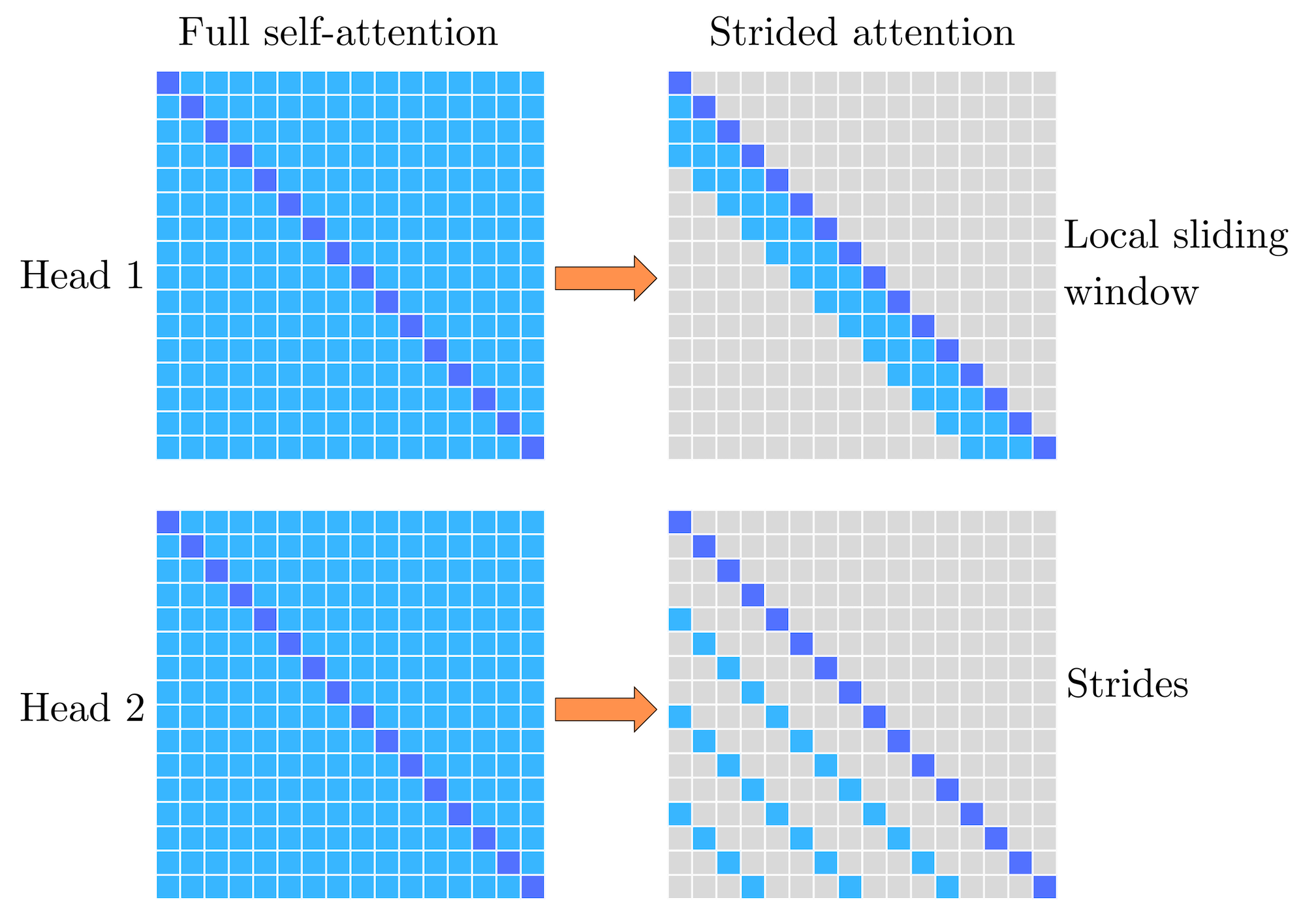
They observed that the strided pattern (attending every k-th position) did not work well for text data, which lacks a naturally periodic structure. As a result, they introduced a fixed attention pattern. In one attention head, the sequence is divided into blocks of fixed size (e.g., 128 tokens). Each token within a block attends only to other tokens in that same block, capturing local dependencies in a more straightforward manner.

However, using purely local attention inside blocks would prevent information from flowing across blocks in deeper layers. To address this, another head connects the "summary token" at the end of each block to the corresponding summary tokens of all previous blocks. Because that last token has attended to all tokens in its own block, its hidden state acts as a summary of that entire sub-sequence. By letting future blocks attend to these summary tokens, the model propagates information globally across blocks, layer by layer.

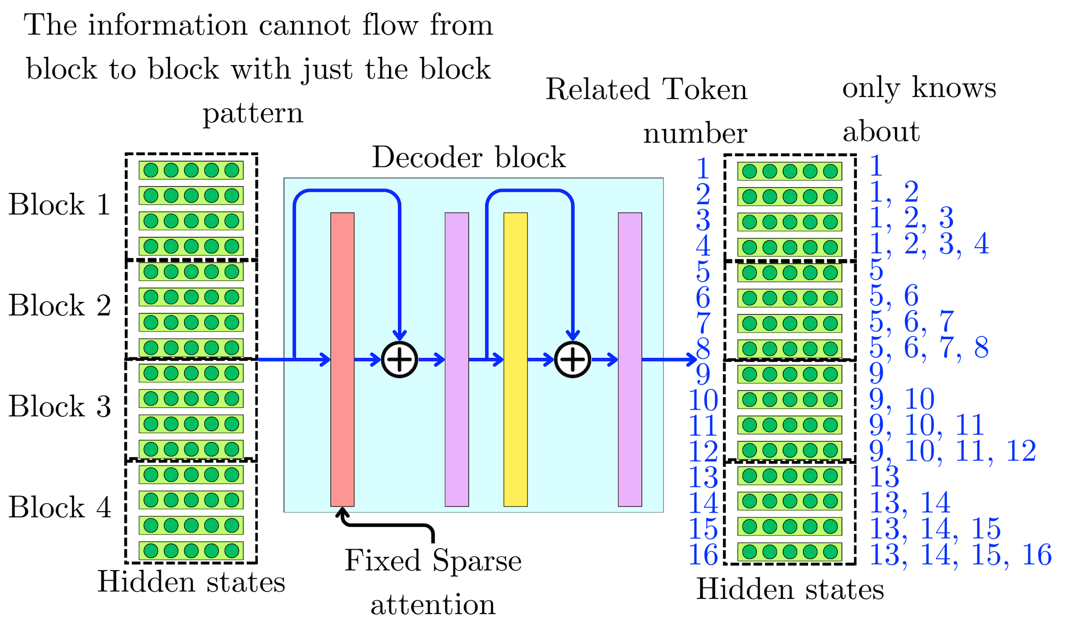
Thus, the in-block pattern computes context vectors (weighted averages of values) only from nearby tokens, while the across-block pattern computes context from previous summary tokens. In combination, these patterns ensure both local and long-range context can be aggregated throughout the Transformer stack, even without a dense (i.e., fully quadratic) attention mechanism.

Let's estimate the time complexity of those sparse attentions. In the strided case, we have a local window of size w and a stride c. Therefore, each query attends to roughly w + N / c keys (the local window plus the strided tokens). For N queries, the total cost is ~ N(w + N / c). By tuning w and c, one can achieve sub-quadratic complexity. For example:

\(\begin{align} N\left(w+\frac{N}{c}\right) \sim \mathcal{O}(N\sqrt{N}), \quad &\text{if }c= \sqrt{N}\nonumber\\ N\left(w+\frac{N}{c}\right) \sim \mathcal{O}(N\log{N}), \quad &\text{if }c=\frac{N} {\log{N}}\nonumber \end{align}\)

In the fixed case, The sequence is split into blocks of length l. Within each block, each query attends at most l keys. Furthermore, each query attends c = N / l summary tokens. Therefore, a query sees O(l + c) keys, and the total cost for all queries is O(N(l + c)). Typically, we choose l such that it grows sub-linearly with N. For example:

\( N(l + c) \sim \mathcal{O}(N\sqrt{N}), \quad \text{if }l= \sqrt{N}\)

Despite the improved time complexity, it is essential for those computations to remain performed as tensor operations to fully utilize the high parallelism of the GPU hardware. For example, let's assume that we want to compute the attentions for the local sliding window described in the strided case. The original keys tensor K is of dimension n_head X d_head X N. We can construct the windowed keys tensor K^w to compute the sliding window all at once by adding another dimension representing the window size w. Constructing this tensor is a O(N) operation. The resulting tensor is of size n_head X d_head X N X w, and each slice of size d_head X N X w contains the necessary keys to compute the windowed attentions for each head.

Let's now compute the product between the windowed keys K^w and the queries Q:

\( E_{hnw}=\sum_{d}\frac{Q_{hdn}K^w_{hdnw}}{\sqrt{d_\text{head}}}, \quad \text{shape: } n_\text{head}\times N\times w\)

where h represents the head dimension (n_head), n the sequence dimension (N), d the hidden size per head dimension (d_head) and w the window dimension. The resulting alignment scores tensor E is of shape n_head X N X w. The time complexity of this operation is O(d_headNw) instead of the vanilla O(d_headN²).

Choosing Sparsity Efficiently: Reformer