Deep Dive: 3 Techniques to take your Machine Learning Model Development to the Next Level

Deep Dive in Data Science Fundamentals

---

There is no end to all the possible techniques you could try when developing a model. It is key to balancing development speed and performance. Over the years, I have found the following techniques to be quite useful to speed up my development while ensuring significant predictive performance gains. We cover the following techniques and implementations:

• The Random Bar technique for Feature Selection

  • The technique

  • Creating synthetic data

  • Tuning the hyperparameters

  • The feature importance

  • The experiment

• The duplication technique for imputing missing values

  • The technique.

  • Create a synthetic dataset

  • Data transformations

  • The experiment

• The expanding mean target encoding to encode categorical variables

  • The technique

  • Generate a synthetic dataset

  • The target encoder

  • The experiment

---

This Deep Dive is part of the Data Science Fundamentals series.

The Random Bar technique for Feature Selection

The Technique

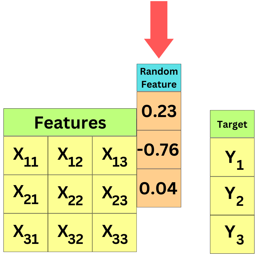
This is a technique I use to perform quick feature selection for Machine Learning applications. I tend to call it the "Random Bar" method! Let's assume you have a feature set X and a target Y. Let's create a random vector V and append it as an additional feature to X:

\(X' = [X, V]\)

X' is just the original feature set plus a new random feature. Keep in mind that this new feature cannot possibly help to predict the target Y since it is random! Now, take that data (X', Y) and train a Supervised Learning algorithm with a Feature Importance measure relevant for your application. Intuitively, the mean entropy gain per split of tree-based algorithms (Random Forest, XGBoost, ...) is a convincing measure of feature importance to me. We know that it is artificial, but even the random feature will be assigned a non-zero value by the algorithm due to the fluctuation in the data. Any feature with a lower feature importance than the random feature has to be useless to predict the target and the features with a higher feature importance are at least better than random noise at predicting the target.

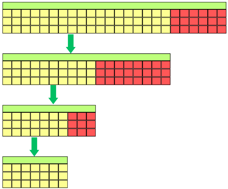
It is likely that the method will not catch all the unnecessary features and multiple iterations may be necessary:

This is especially useful if you have thousands of features and you want to weed out quickly the ones that won't have any impact on the learning process. This is also a method that can be used for highly non-linear data unlike LASSO (for example) which tends to only understand linear relationships in the data. The random feature is a "Random Bar" because this is the minimum bar a feature needs to beat to be a part of a potentially useful feature set. However, it does not mean you can't further optimize your model by removing additional features.

Creating synthetic data

Let’s first create a difficult dataset to learn from. We use the make_classification function from Scikit-Learn to create a synthetic dataset. We set it up with 10,000 samples and 1,000 features. We make it a binary classification problem and set the number of informative variables to 20:

from sklearn.datasets import make_classification
from sklearn.model_selection import train_test_split

def get_data():
    X, y = make_classification(
        n_samples=10000,
        n_features=1000,
        n_informative=20,
        n_classes=2,
        class_sep=0.001,
        n_clusters_per_class=4,
    )

    # we split the data into train and val sets
    X_train, X_val, y_train, y_val = train_test_split(
        X, y, test_size=0.25
    )
    return X_train, X_val, y_train, y_val 

X_train, X_val, y_train, y_val = get_data()
X_train

We create a function to add the random bar to the feature set:

import numpy as np

def add_random_bar(X):

    # we create a random vector with as many samples as the 
    # the data 
    random_col = np.random.normal(size=(X.shape[0], 1))

    # we append this new feature to the feature set
    X = np.concatenate((X, random_col), 1)
    return X

Tuning the hyperparameters

We use XGBoost as a learner to compute feature importance. We use Bayesian Optimization to tune the hyperparameters at each iteration. Check out this deep dive if you need a refresher on Bayesian Optimization:

This time, we use BayesSearchCV from scikit-optimize. We write the function that returns the optimal hyperparameters

from xgboost import XGBClassifier
from skopt import BayesSearchCV

def tune_hyperparameters(X_train, y_train, X_val, y_val):

    # we set up the classifier we want to tune. We use early 
    # stopping after 10 iteration. We use 'binary:logistic'
    # to make it a binary classifier. We use 'auc' as the 
    # evaluation metric for early stopping. 
    clf = XGBClassifier(
        n_estimators=1000,
        early_stopping_rounds=10,
        objective='binary:logistic', 
        eval_metric='auc',
        n_jobs=-1
    )
    
    # we set up the optimizer with the classifier and its
    # search-space
    opt = BayesSearchCV(
        clf,
        {
            'eta':  (0.0, 1.0, 'uniform'),
            'gamma': (0.0, 50, 'uniform'),
            'max_depth': (1, 15),
            'min_child_weight': (0.0, 10.0, 'uniform'),
            'max_delta_step': (0.0, 10.0, 'uniform'),
            'subsample': (0.0, 1.0, 'uniform'),
            'lambda': (0.0, 5.0, 'uniform'),
            'alpha': (0.0, 5.0, 'uniform')   
        },
        n_iter=32,
        cv=3,
    )
    
    opt.fit(
        X_train, 
        y_train,
        eval_set=[(X_val, y_val)]
    )
    
    # we return the optimal hyperparameters
    return opt.best_params_

The feature importance