GBM vs XGBoost vs LightGBM vs CatBoost

• The Bias-Variance Tradeoff

• The Gradient Boosted Trees Algorithm

• How to build trees in XGBoost

• LightGBM

• CatBoost

---

The Bias-Variance Tradeoff

XGBoost was developed by Tianqi Chen in 2014 in the original paper XGBoost: A Scalable Tree Boosting System. It has a lot of advantages:

• Highly performant model

• Handle missing values

• It is parallelizable

• Robust to overfitting on the number of features

Before we can dig into it, let’s consider the concept of bias and variance tradeoff.

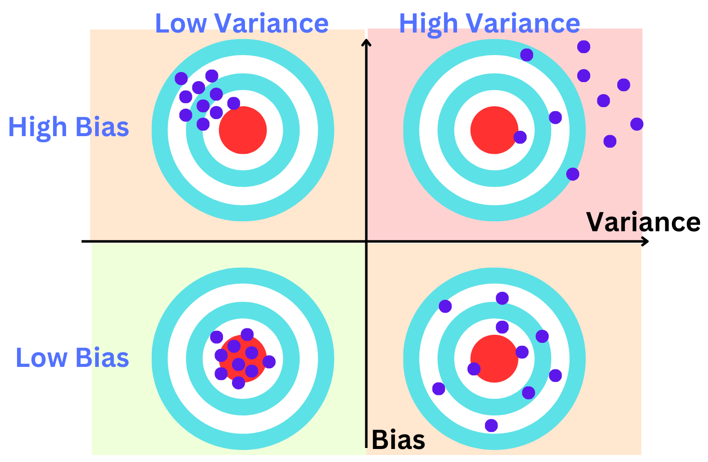
A low-bias machine learning model refers to a model that does not make strong assumptions about the form of the underlying data distribution. This is in contrast to a high-bias model, which makes significant assumptions about the data structure:

1. Assumptions About Data: Low-bias models are flexible and can adapt to a wide variety of data shapes and structures. They do not assume that the data follows a specific distribution or pattern. High-bias models, on the other hand, are based on strong assumptions about the data's distribution. For example, a linear regression model assumes that the relationship between variables is linear.

2. Overfitting and Underfitting: Low-bias models have a lower risk of underfitting the data, meaning they are usually better at capturing the true relationships in the data, including complex and nuanced patterns. However, they can be prone to overfitting, where the model fits the training data too closely and performs poorly on new, unseen data. High-bias models are more likely to underfit as they might oversimplify the data, missing important trends or patterns.

3. Flexibility: Low-bias models are typically more complex and flexible, allowing them to adjust to various data types and structures. This complexity can come at the cost of interpretability and computational efficiency.

4. Examples of Low-Bias Models: Examples of low-bias machine learning models include Decision Trees, Random Forests, and Neural Networks. These models do not make strong assumptions about the data and can model complex relationships.

5. Generalization: The primary goal with low bias models is to achieve good generalization, meaning they perform well not only on the training data but also on new, unseen data. This requires careful tuning to avoid overfitting.

The difference between low and high variance in machine learning models fundamentally relates to how sensitive these models are to fluctuations in the training data:

1. Sensitivity to Training Data:

   • Low Variance Models: They are not very sensitive to small changes or noise in the training data. When trained on different subsets of the data, a low-variance model will produce similar results. This consistency makes them more predictable but can lead to underfitting, where the model oversimplifies the data and misses important patterns.

   • High Variance Models: These models are highly sensitive to fluctuations in the training data. They can capture subtle and complex patterns in the data, but this also means they might capture noise as a meaningful signal (overfitting). When trained on different subsets of data, high-variance models can yield widely varying results.

2. Generalization:

   • Low Variance Models: They tend to generalize better to unseen data as they are less likely to overfit the training data. However, if they are too simple (high bias), they might not perform well even on new data due to their inability to capture the complexity of the data.

   • High Variance Models: While they can perform exceptionally well on the training data by capturing intricate patterns, their performance on new, unseen data can be poor if they've overfitted. They require careful tuning, often needing larger datasets and techniques like regularization to generalize well.

3. Complexity and Flexibility:

   • Low Variance Models: These are typically simpler, less complex models. Examples include linear models like Linear Regression. Their simplicity contributes to their stability but limits their flexibility.

   • High Variance Models: Such models are often more complex and flexible. They can adapt to a wide variety of data patterns. Examples include models like Decision Trees, Random Forests, and Neural Networks.

4. Bias-Variance Tradeoff:

   • In machine learning, there's an essential tradeoff between bias and variance. Low variance models often have high bias, meaning they make strong assumptions about the data and may not capture its true complexity. High variance models usually have low bias, being more flexible and capable of capturing complex relationships in the data, but at the risk of overfitting.

Algorithms like Linear Regression have their number of degrees of freedom (d.o.f. - complexity) scaling with the number of features O(M). In practice, this means that their ability to learn from the data will plateau in the regime N >> M, where N is the number of samples (typically large data sets). They have a high bias but a low variance, and as such, they are well adapted to the N > M regime. In the N < M regime, L1 regularization becomes necessary to learn the relevant features and zero out the noise (think about having more unknowns than equations to solve a set of linear equations). Naive Bayes d.o.f. scales as O(C x M) (or O(M) depending on the implementation), where C is the number of categories the features are discretized into. O(C) = O(N) in theory but not really in practice. This makes it a lower bias algorithm than LR, but it is a product ensemble of univariate models and ignores the feature interactions (as LR does), preventing it from further improvements. 

A tree in its unregularized form, is a low bias algorithm (you can overfit the data to death), with d.o.f scaling as O(N), but high variance (deep trees don’t generalize well). But because a tree can reduce its complexity as much as needed, it can work in the regime N < M by simply selecting the necessary features. A Random Forest is,, therefore,, a low-bias algorithm, but the ensemble averages away the variance (but deeper trees call for more trees), and it doesn’t overfit on the number of trees (Theorem 1.2 in the classic paper by Leo Breiman), so it is a lower variance algorithm. The homogenous learning (the trees tend to be similar) tends to limit its ability to learn on too much data.  

XGBoost is the first (to my knowledge) tree algorithm to mathematically formalize regularization in a tree (eq. 2 in the XGBoost paper). It has a low bias and high variance (due to the boosting mechanism) and is therefore adapted to large data scales. The GBM Boosting mechanism ensures more heterogeneous learning than Random Forest and, therefore, adapts better to larger scales. The optimal regularization ensures higher quality trees as weak learners than in Random Forest and tends to be more robust to overfitting than Random Forest.   

In the regime N >> M, only low-bias algorithms make sense with d.o.f. scaling as O(N). That includes algorithms like GBM, RF, Neural Networks, SVM (gaussian), KNN,… SVM has a training time complexity of O(N^3) (unmanageable!), and KNN is bad at understanding what an important feature is and has dimensionality errors scaling as O(M). Neural Networks are known to underperform compared to XGBoost on tabular data ("Deep Learning is not all you need"). 

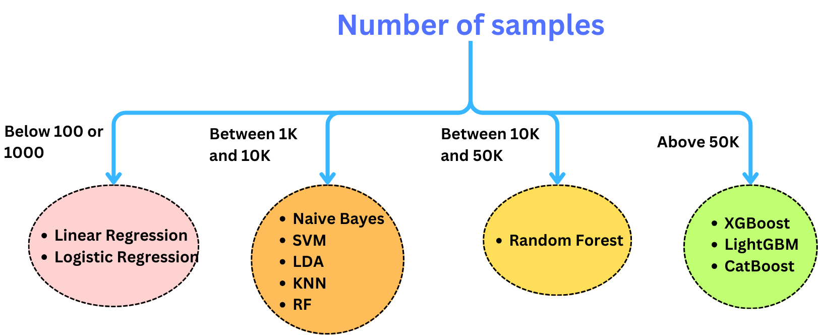
Here is a rule of thumb to choose an initial model based on the size of the data:

The Gradient Boosted Trees Algorithm