Introduction to Deep Learning

• The Computational Graph

• The Back-propagation algorithm

• The Optimizers

• The Activation Functions

• The Regularization strategies

• The Computational Blocks

---

The Computational Graph

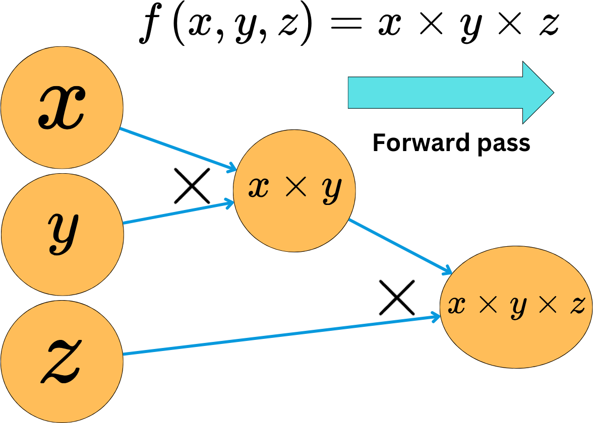
One important aspect of Deep Learning is the need to compute the derivatives of complex functions efficiently. In neural network frameworks like PyTorch, this is handled by storing the operations and variables of functions on a computational graph. Nodes represent the variables, and the edges represent operations. An incoming edge means a new variable has been created by applying an operation on other variables.

Creating the graph and computing the values at the different nodes is called the forward pass.

For each operation we apply, we know the derivative rules for the different variables involved, so we can easily compute the derivatives of the output variables as a function of the input variables. For a specific node, we only need to compute the derivatives of the outgoing variable with respect to the incoming variables. By applying the derivative chain rule, we can compute the derivatives of the output variables with respect to input variables for the whole graph. At every point of the process, we only compute the basic derivatives for a triplet of variables, but the chain rule allows us to compute derivatives for extremely complex functions.

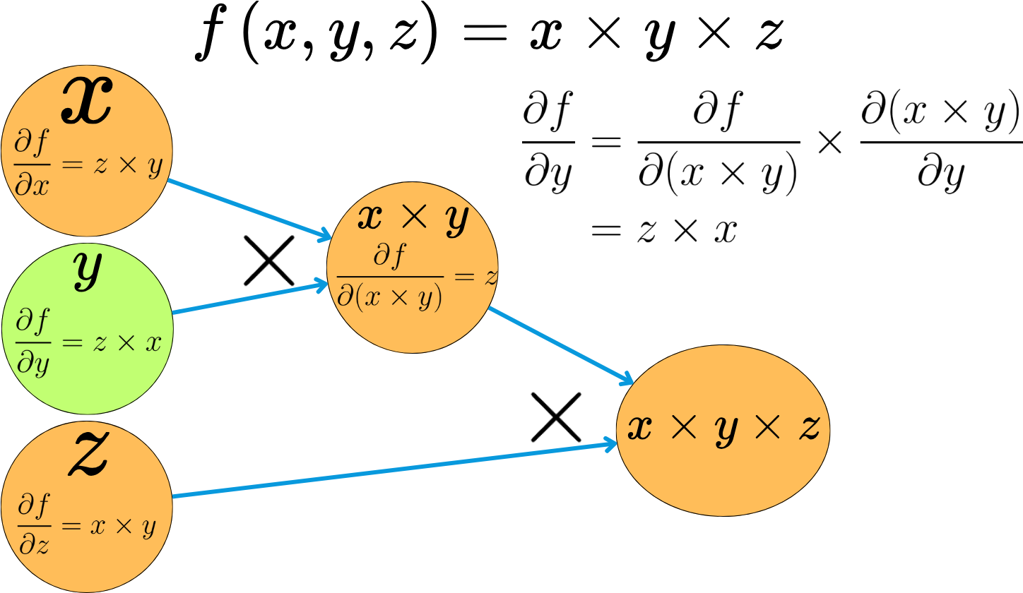
Back-propagating the derivatives at the inputs of the graph is referred to as the backward pass.

We can easily implement this in PyTorch:

import torch

x = torch.tensor([2.0], requires_grad=True)
y = torch.tensor([3.0], requires_grad=True)
z = torch.tensor([4.0], requires_grad=True)

# Perform the operation
f = x * y * z  # f(x, y, z) = x * y * z

# Compute gradients
f.backward()

# Gradients: df/dx = y * z, df/dy = x * z, df/dz = x * y
print(f"Gradient df/dx: {x.grad}")  # Output should be 3.0 * 4.0
print(f"Gradient df/dy: {y.grad}")  # Output should be 2.0 * 4.0
print(f"Gradient df/dz: {z.grad}")  # Output should be 2.0 * 3.0

> Gradient df/dx: tensor([12.])
> Gradient df/dy: tensor([8.])
> Gradient df/dz: tensor([6.])

We can have complex computational blocks and still easily backpropagate the derivatives.

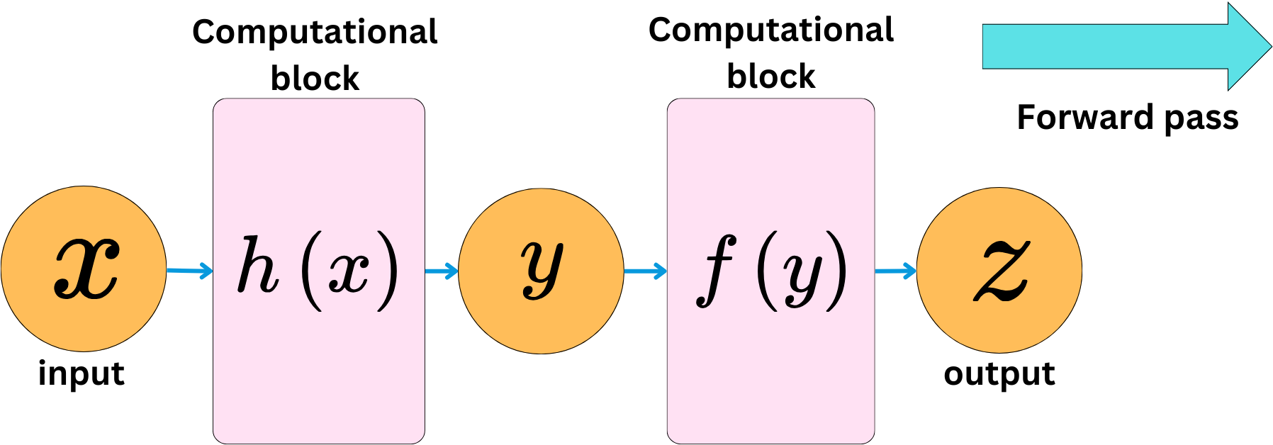
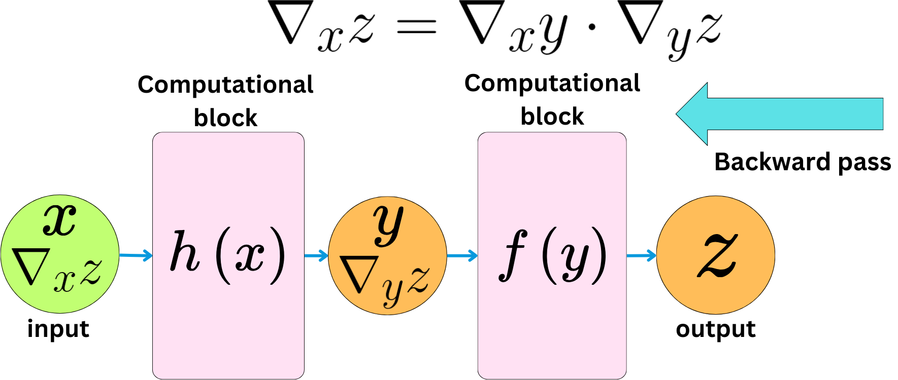
The chain rule will always reduce the problem to a simple product operation. The backward pass is about computing the gradient of the output with respect to the inputs.

For example, in PyTorch:

def h(x):
    return x**2

def f(y):
    return y + 1


# Define tensors
x = torch.tensor(2.0, requires_grad=True)

# Define the computational blocks
y = h(x)  # Some function h
z = f(y)  # Some function f

# Compute gradients
z.backward()

# x.grad will contain ∇_{x}z
print("Gradient of z with respect to x:", x.grad)

> Gradient of z with respect to x: tensor(4.)

The network and the related functional relationship between the inputs and outputs can be as complex as we want.

Computing the derivatives (gradients) will always reduce to computing simple products due to the chain rule.

The Back-propagation algorithm